Continuing our deep dive into Jet's fundamentals we shall now move on to infinite stream processing. The major challenge in batch jobs was properly parallelizing/distributing a "group by key" operation. To solve it we introduced the idea of partitioning the data based on a formula that takes just the grouping key as input and can be computed independently on any member, always yielding the same result. In the context of infinite stream processing we have the same concern and solve it with the same means, but we also face some new challenges.
Stream Skew
We already introduced the concept of the watermark and how it imposes order onto a disordered data stream. Items arriving out of order aren't our only challenge; modern stream sources like Kafka are partitioned and distributed so "the stream" is actually a set of independent substreams, moving on in parallel. Substantial time difference may arise between events being processed on each one, but our system must produce coherent output as if there was only one stream. We meet this challenge by coalescing watermarks: as the data travels over a partitioned/distributed edge, we make sure the downstream processor observes the correct watermark value, which is the least of watermarks received from the contributing substreams.
Sliding and Tumbling Window
Many quantities, like "the current rate of change of a price" require you to aggregate your data over some time period. This is what makes the sliding window so important: it tracks the value of such a quantity in real time.
Calculating a single sliding window result can be quite computationally intensive, but we also expect it to slide smoothly and give a new result often, even many times per second. This is why we gave special attention to optimizing this computation.
We optimize especially heavily for those aggregate operations that have a cheap way of combining partial results and even more so for those which can cheaply undo the combining. For cheap combining you have to express your operation in terms of a commutative and associative (CA for short) function; to undo a combine you need the notion of "negating" an argument to the function. A great many operations can be expressed through CA functions: average, variance, standard deviation and linear regression are some examples. All of these also support the undoing (which we call deduct). The computation of extreme values (min/max) is an example that has CA, but no good notion of negation and thus doesn't support deducting.
This is the way we leverage the above properties: our sliding window actually "hops" in fixed-size steps. The length of the window is an integer multiple of the step size. Under such a definition, the tumbling window becomes just a special case with one step per window.
This allows us to divide the timestamp axis into frames of equal length and assign each event to its frame. Instead of keeping the event object, we immediately pass it to the aggregate operation's accumulate primitive. To compute a sliding window, we take all the frames covered by it and combine them. Finally, to compute the next window, we just deduct the trailing frame and combine the leading frame into the existing result.
Even without deduct the above process is much cheaper than the most naïve approach where you'd keep all data and recompute everything from scratch each time. After accumulating an item just once, the rest of the process has fixed cost regardless of input size. With deduct, the fixed cost approaches zero.
Example: 30-second Window Sliding by 10 Seconds
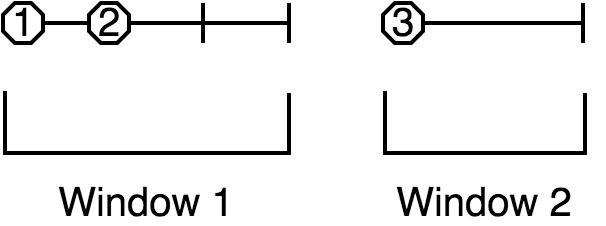
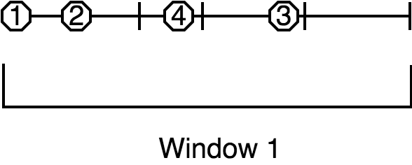
We'll now illustrate the above story with a specific example: we'll construct a 30-second window which slides by 10 seconds (i.e., three steps per window). The aggregate operation is to simply count the number of events. In the diagrams we label the events as minutes:seconds. This is the outline of the process:
- Throw each event into its "bucket" (the frame whose time interval it belongs to).
- Instead of keeping the items in the frame, just keep the item count.
- Combine the frames into three different positions of the sliding window, yielding the final result: the number of events that occurred within the window's timespan.
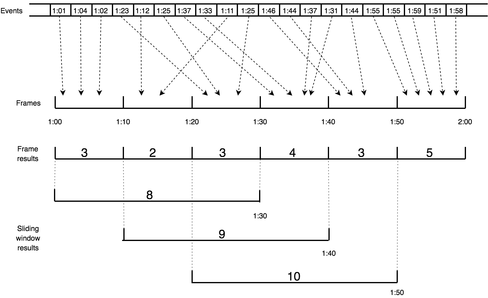
This would be a useful interpretation of the results: "At the time 1:30, the 30-second running average was 8/30 = 0.27 events per second. Over the next 20 seconds it increased to 10/30 = 0.33 events per second."
Keep in mind that the whole diagram represents what happens on just one cluster member and for just one grouping key. The same process is going on simultaneously for all the keys on all the members.
Two-stage aggregation
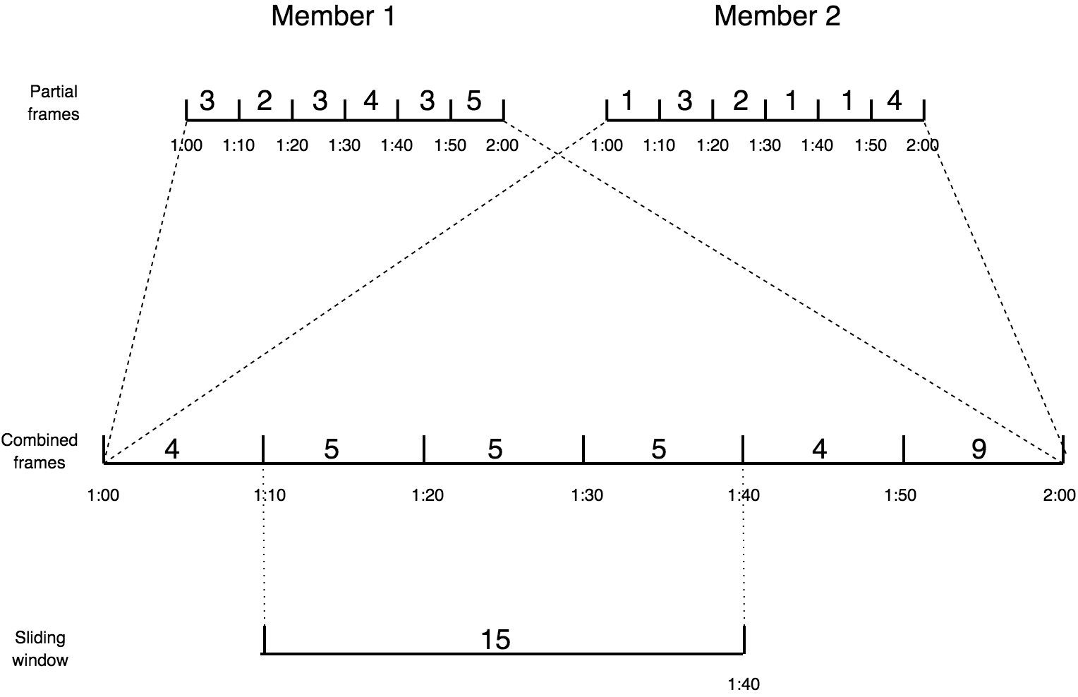
The concept of frame combining helps us implement two-stage aggregation as well. In the first stage the individual members come up with their partial results by frame and send them over a distributed edge to the second stage, which combines the frames with the same timestamp. After having combined all the partial frames from members, it combines the results along the event time axis into the sliding window.
Session Window
In the abstract sense, the session window is a quite intuitive concept: it simply captures a burst of events. If no new events occur within the configured session timeout, the window closes. However, because the Jet processor encounters events out of their original order, this kind of window becomes quite tricky to compute.
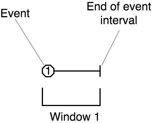
The way Jet computes the session windows is easiest to explain in terms
of the event interval: the range
[eventTimestamp, eventTimestamp + sessionTimeout].
Initially an event causes a new session window to be created, covering
exactly the event interval.
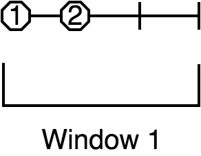
A following event under the same key belongs to this window iff its interval overlaps it. The window is extended to cover the entire interval of the new event.
If the event intervals don't overlap, a new session window is created for the new event.
An event may happen to belong to two existing windows if its interval bridges the gap between them; in that case they are combined into one.
Once the watermark has passed the closing time of a session window, Jet can close it and emit the result of its aggregation.
Distributed Snapshot
The technique Jet uses to achieve fault tolerance is called a "distributed snapshot", described in a paper by Chandy and Lamport. At regular intervals, Jet raises a global flag that says "it's time for another snapshot". All processors belonging to source vertices observe the flag, create a checkpoint on their source, and emit a barrier item to the downstream processors and resumes processing.
As the barrier item reaches a processor, it stops what it's doing and emits its state to the snapshot storage. Once complete, it forwards the barrier item to its downstream processors.
Due to parallelism, in most cases a processor receives data from more than one upstream processor. It will receive the barrier item from each of them at separate times, but it must start taking a snapshot at a single point in time. There are two approaches it can take, as explained below.
Exactly-Once Snapshotting
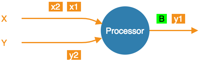
With exactly-once configured, as soon as the processor gets a barrier item in any input stream (from any upstream processor), it must stop consuming it until it gets the same barrier item in all the streams:
- At the barrier in stream X, but not Y. Must not accept any more X items.
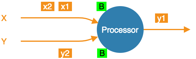
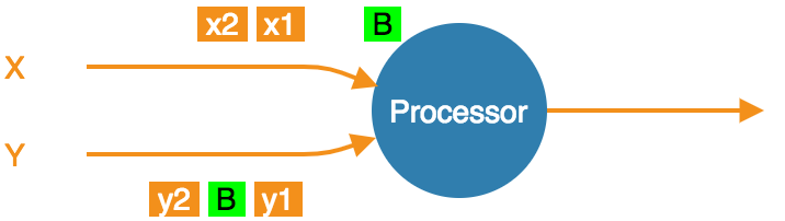
- At the barrier in both streams, taking a snapshot.
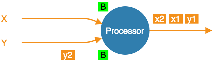
- Snapshot done, barrier forwarded. Can resume consuming all streams.
At-Least-Once Snapshotting
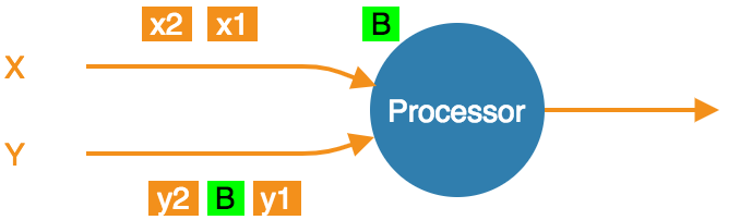
With at-least-once configured, the processor can keep consuming all the streams until it gets all the barriers, at which point it will stop to take the snapshot:
- At the barrier in stream X, but not Y. Carry on consuming all streams.
- At the barrier in both streams, already consumed
x1andx2. Taking a snapshot.
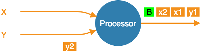
- Snapshot done, barrier forwarded.
Even though x1 and x2 occur after the barrier, the processor
consumed and processed them, updating its state accordingly. If the
computation job stops and restarts, this state will be restored from the
snapshot and then the source will replay x1 and x2. The processor
will think it got two new items.
The Pitfalls of At-Least-Once Processing
In some cases at-least-once semantics can have consequences of quite an unexpected magnitude, as we discuss next.
Apparent Data Loss
Imagine a very simple kind of processor: it matches up the items that belong to a pair based on some rule. If it receives item A first, it remembers it. Later on, when it receives item B, it emits that fact to its outbound edge and forgets about the two items. It may also first receive B and wait for A.
Now imagine this sequence: A -> BARRIER -> B. In at-least-once the
processor may observe both A and B, emit its output, and forget about
them, all before taking the snapshot. After the restart, item B will be
replayed because it occurred after the last barrier, but item A won't.
Now the processor is stuck forever in a state where it's expecting A and
has no idea it already got it and emitted that fact.
Problems similar to this may happen with any state the processor keeps until it has got enough information to emit the results and then forgets it. By the time it takes a snapshot, the post-barrier items will have caused it to forget facts about some pre-barrier items. After a restart it will behave as though it has never observed those pre-barrier items, resulting in behavior equivalent to data loss.
Non-Monotonic Watermark
One special case of the above story concerns watermark items. Thanks to watermark coalescing, processors are typically implemented against the invariant that the watermark value always increases. However, in at-least-once the post-barrier watermark items will advance the processor's watermark value. After the job restarts and the state gets restored to the snapshotted point, the watermark will appear to have gone back, breaking the invariant. This can again lead to apparent data loss.